Setting Robust Process Specifications Using Design of Experiments and Monte Carlo Techniques
Abstract
Setting specifications on process parameters can be a difficult job. Setting robust specifications that won't need constant adjustment may seem almost impossible. This presentation will show how a combination of Design of Experiments and Monte Carlo techniques can be used to set robust process specifications in a straightforward, objective manner. You will see an example using published data for a rubber manufacturing process. You will see the stages from designing an experiment for optimizing the process specifications through the use of a Monte Carlo simulator to study the responses to specification changes. You will see these results used to optimize the process specifications. You won't need to delve into the math -- the software JMP will handle that. You will leave this presentation with a new paradigm for setting robust process parameter specifications.
Introduction
Setting specifications on process parameters can be a difficult job. Setting robust specifications that won't need constant adjustment may seem almost impossible.
Here is a typical scenario: manufacturing requests specifications on the process parameters for a new product from the development team. No one on the team really knows what these limits should be. Realistic specifications are everyone's desire, but with no knowledge of how to set realistic specs, development usually opts to protect their reputation by setting specs so tight that they are guaranteed to work. Unfortunately, this makes life more difficult for manufacturing and development. Each time a particular lot of product does not meet spec, manufacturing must ask development if this product is really OK to sell. Development must investigate. If it determines that this product is OK to sell, the specifications are modified to allow for this difference in the future. This may happen several times before the specs are widened to realistic limits.
Robust specifications are realistic. They don't require this labor intensive iterative changing of specs. They are correct, or very nearly so, right from the start.
Here's the good news – you can use data to set robust specifications that are realistic. The key is the use of an empirical model to predict the consequences of different specification choices.
The Objective Design of Experiments 7-Step Process for experimentation will provide this empirical model. Monte Carlo analysis on this model will elucidate the consequences of the specification choices. The Seven Steps to Build an Empirical Model
- Ask the Right Question
- Choose your model
- Choose an Experiment Design
- Collect Your Data
- Analyze Your Data
- Test Model (Including Specification Scenarios)
- Celebrate Success! (Take Pride in a Job Well-Done)
We will discuss each of these steps as it applies to setting specifications.
Step 1. Ask the right question
Voice of the Customer – The customer requires “durable” truck tires. Durable needs to be clarified to insure that we can satisfy the customer. This can be an involved and time-consuming step, but ultimately researchers determined that a substitute quality characteristic that can be measured and that correlates with durability was needed.
Substitute Quality Characteristic – Modulus 300 was chosen to substitute for durability. Maximizing Modulus 300 should also maximize durability. Modulus 300 is relatively easy to measure and provides numbers for our analysis.
Goals – It is believed that if we can keep the Modulus 300 greater than 160 we will have a sufficiently durable tire. We would prefer to have a Modulus 300 of 180 or greater if possible.
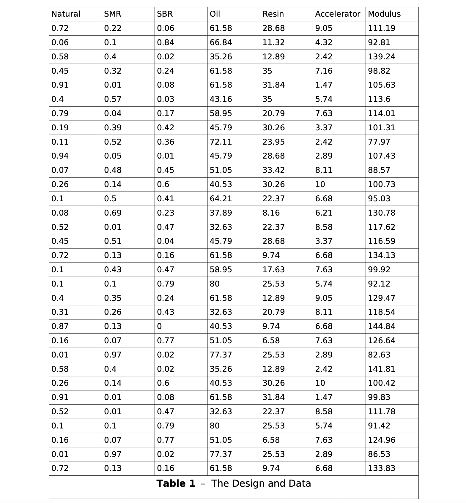
Select Factors and Limits – Selecting which factors to study and which to hold constant can be a very involved project. It may involve examination of existing theories, evaluation of existing data, and the application of screening experiments. Time does not permit a detailed analysis of factor selection here, but researchers determined that three components and three additives were potentially important to the rubber formulation:
Rubber components:
- Natural rubber 0 – 100%
- SMR rubber 0 - 100%
- SBR rubber 0 - 100%
Additives:
- Oil 30 – 80 g/kg
- Resin 5 – 35 g/kg
- Accelerator 1 – 10 g/kg
Also, several additional additives will be added at constant levels: sulfur, zinc oxide, stearic acid, and carbon black. While these ingredients are necessary, they are not thought to have any significant effect on durability.
Step 2: Choose a Model
We need a model to predict the behavior of our rubber formulation. We don't know the true model. The theoretical background alone is inadequate to formulate a mathematical model. Where do we go from here?
Fortunately, mathematician Brook Taylor discovered the answer in the time of Newton. Taylor's theorem tells us that we can approximate any smooth, continuous function using a polynomial. So, whatever the real model looks like, we can fit our data to a polynomial to predict future behavior. (Of course we will have to test this model to make sure it will predict well – that will come in step 6.)
The specific polynomial we used is listed below:
Modulus 300 = b1Natural + b2SMR + b3SBR + b12Natural * SMR + b13NaturalSBR + b14NaturalOil + b15NaturalResin + b16NaturalAccelerator + b23SMRSBR + b24SMROil + b25SMRResin + b26SMRAccelerator + b34SBROil + b35SBRResin + b36SBRAccelerator + b45OilResin + b46OilAccelerator + b56ResinAccelerator + b44Oil ^2 + b55Resin ^2 + b66*Accelerator ^2
The “b's” are coefficients that adjust the model to fit the data we will collect. b1 through b3 model the “main effects” of our components – the effect each factor has on Modulus 300. b44,b55, and b56 model curvature in the effect of Modulus 300. b12 through b56 model interactions among factors, allowing us to see what happens if these factors change together. With our model specified, we need to know what data to collect to fit this model best.
Step 3: Choose an Experiment Design
An experiment design will provide us with a list of the best experiments to run to collect data to fit our model. The list will be efficient and maximize the quality of the fit.
We have specified a customized model to work around experimental constraints. Because of this, no design is available in the literature. We will need to create a custom design for our model.
Fortunately, mathematicians Jack Kiefer and Jacob Wolfowitz discovered a brilliant way to specify experiment designs that maximizes the quality of fit in industrial situations. Even more fortunately, JMP provides an algorithm for the routine generation of I-Optimal Designs.
We can use JMP to create a custom experiment design for our model.
Step 4: Collect Data
Establishing a cause-effect relationship requires that every factor be accounted for. This is not so easy. It may not even be possible to identify all of the factors influencing our work.
Fortunately again, the field of Statistics provides us with a way to account for all of the factors:
- Include the most important factors in the experiment design.
- Hold other known factors constant.
- Execute experimental runs in a random order. (This forces any remaining, uncontrolled factors to look like noise so we can account for these effects in our uncertainty).
We used all three steps above to insure that the effects we observed were actually caused by the factors we were varying.
Step 5: Analyze the Data
The first step in the analysis is to check to see if the standard deviation is constant (homogeneous variance) over the range of our experimental trials. The analysis, not shown, indicates constant standard deviation.
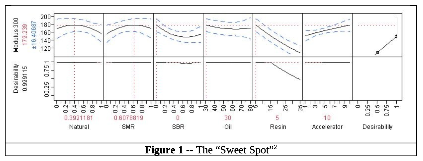
The model was built from the data. Figure 1 shows the behavior of Modulus 300 around the “Sweet Spot” – the combination of factors yielding the best performance. Note that dotted vertical lines indicate the Sweet Spot to be at about 39% Natural rubber, 61% SMR rubber, 30 g/kg Oil, 5 g/kg Resin, and 10 g/kg Accelerator. Note also that the predicted Modulus 300 at this Sweet Spot is about 179.
Step 6: Test the Model and the Sweet Spot
Test the Model - The model was tested in the lab at the Sweet Spot. The predicted response is 179 ± 17. The Modulus 300 measured in the lab was 170.4. Thus the measurement is within the uncertainty of the prediction, indicating a good prediction.
#Test the Sweet Spot* - The Sweet Spot was run in the lab several times and the Statistical Tolerance limits were calculated as shown in Table 2. Notice that the mean is 5.5 less than the prediction. This is a high bias in the model that we can adjust for.

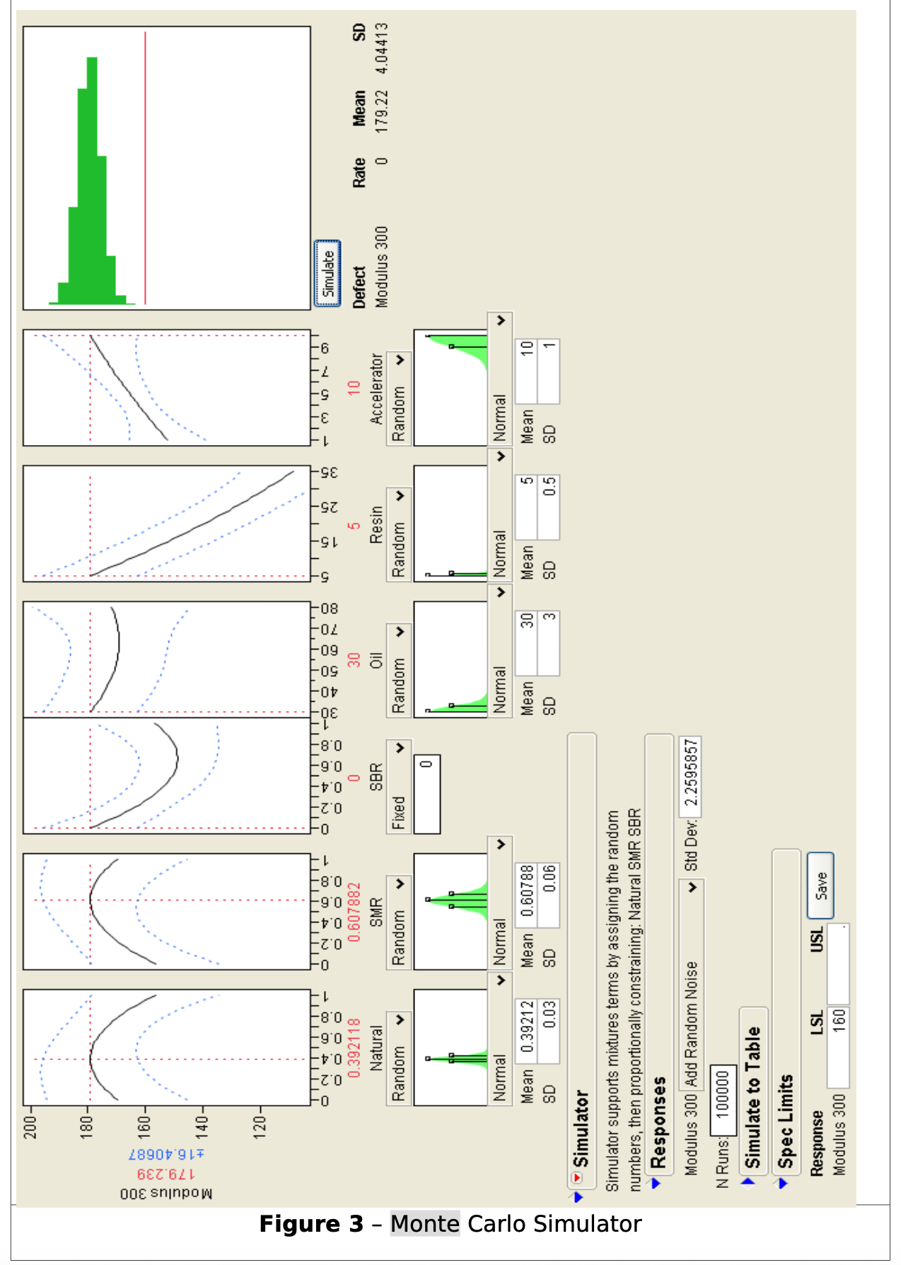
Monte Carlo Analysis to Elucidate the Consequences of the Specifications – As a first pass, let's look at what would happen if the specs assumed a relative standard deviation of 10% for all factors. The nominal factor levels are the Sweet Spot levels, namely 39% Natural rubber, 61% SMR rubber, no SBR rubber, 30 g/kg oil, 5 g/kg resin, and 10 g/kg accelerator. Figure 3 shows the JMP output for the Monte Carlo simulation. Notice that each factor is sampled from a normal distribution with a standard deviation of 10% of the mean value. Notice also that random noise (the noise seen during experimentation) is being included. The histogram in the upper right corner shows the expected Modulus 300 distribution. The red line indicates the lower specification limit of 160.
The histogram of Modulus 300 looks good compared to the lower specification limit. However, remember that the model is biased a little bit high at the Sweet Spot, so we need to correct for that. It would also be nice to know the expected CPK if we went into production with these specifications.
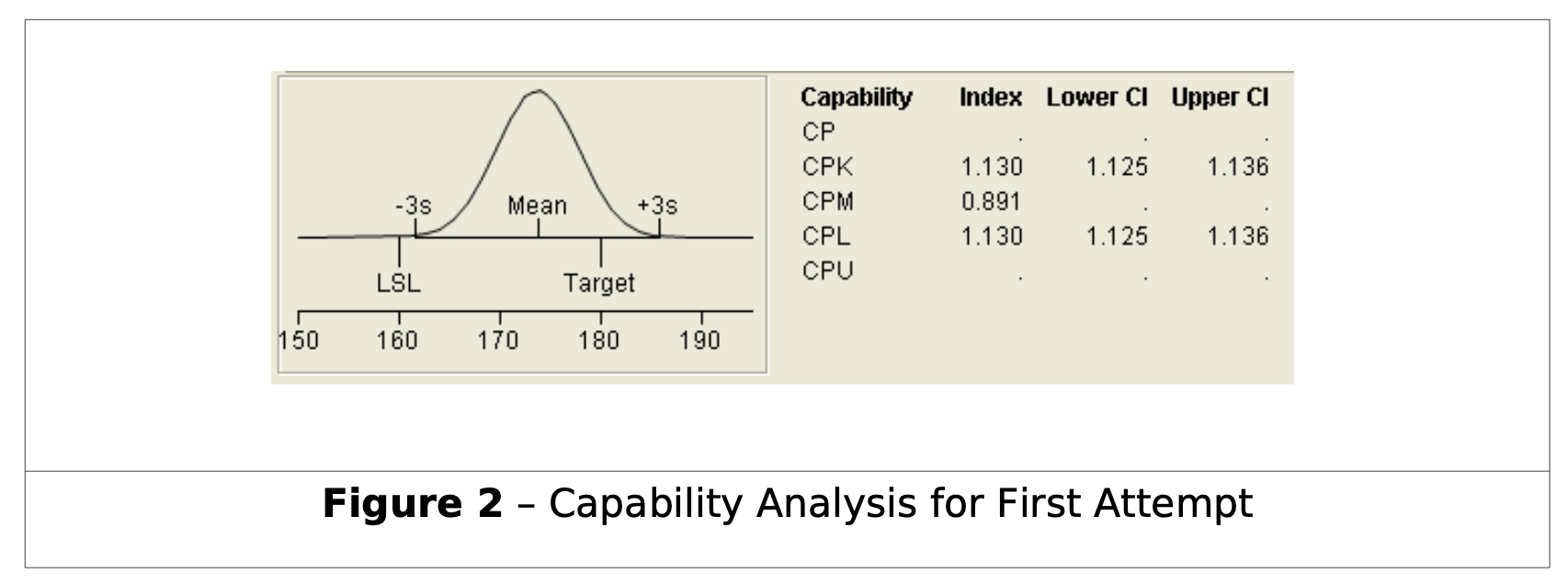
Saving the simulated responses to a data table will allow us to accomplish these tasks. Click on the “Simulate to Data Table” button. In the resulting table, create a new column for corrected Modulus 300. In this column add a formula to reduce each predicted Modulus 300 by 5.5 to correct for the bias. Next, perform a capability analysis on the corrected Modulus 300 data. The result is shown in Figure 2.
A CPK of 1.13 is not good enough. We need to achieve at least 1.3.
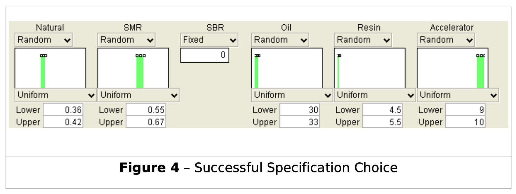
What would happen if we could maintain a specification of ± 10% as a range, instead of as the Standard Deviation? The set up for this is in Figure 4. We will simulate with a Uniform Distribution instead of a Normal distribution. As before, we will simulate to a data table, correct for bias, and perform a capability analysis. The result is in Figure 5.
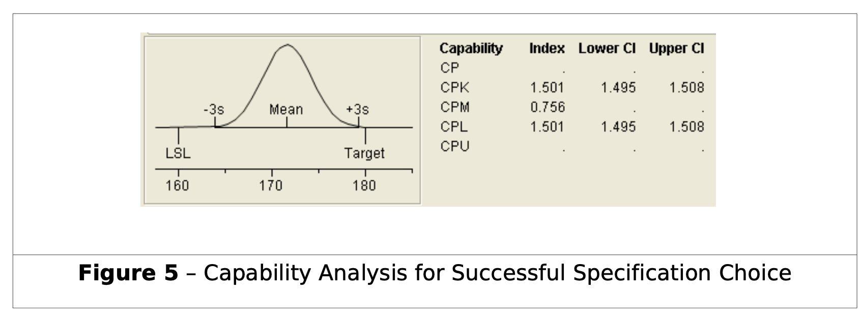
The CPK of 1.5 is very nice. These specifications should produce consistently durable rubber. Tolerance limits show that 99% of rubber produced under these specifications should have a Modulus 300 above 165 with 95% confidence. Now we need to work with manufacturing to meet these specifications.
Step 7: Celebrate Success! (Take Pride in a Job Well-Done)
Now it's time to take pride in a job well done! You have used your budget wisely and carefully. Your specifications are data-driven, not luck-driven. Be sure to celebrate this in some way.
Conclusion
Design of Experiments methodology was used to set robust specifications for rubber manufacture. A seven-step process was used to guide the experiment, analysis, and implementation. Monte Carlo simulation was used to test the consequences of various specification choices.
Looking for More?
Here are some interesting references for further information:
- Box, Hunter, and Hunter, Statistics for Experimenters, J. Wiley and Sons, 1978, ISBN 0-471-09315-7, pp. 307-319.
- Vuchkov, Damgaliev, and Yontchev, “Sequentially Generated Second Order Quasi D-Optimal Designs for Experiments with Mixture and Process Variables,” Technometrics, Vol. 23, No. 3, August 1981, pps 223 – 238. (for information on the rubber example)
- Sobol, Ilya M, A primer for the Monte Carlo Method, CRC Press, 1994, ISBN 0-8493-8673-X