Everything You've Always Wanted to Know About the Weibull Distribution but Were Afraid to Ask!
Background
The Weibull distribution is used to describe the time to failure of parts. These can be transistors, printers, lasers, or even people. The Weibull is popular due to its flexibility. A wide range of physical phenomena can be predicted very well with it.
The life times of parts (or people) are not all identical. Times to failure pile up mostly around some average, with fewer observations at shorter and longer times. If we make a bar graph of the frequency of the life times, we get something called a histogram. The life times are said to follow a distribution, because they are distributed (spread out). The shape of the histogram will depend on what is being studied. If parts fail according to a Weibull distribution, the probability that any single part will fail by a particular time, t, is
F(t) = 1 – exp[-(t/a)^b]
where “a” is called the scale parameter, “b” is called the shape parameter, and F is called the cumulative distribution function (cdf). If we knew a and b, then we could plug them into the function above and calculate F(t). The values of a and b are estimated from the data. The Weibull distribution is called “parametric” because the probability depends on the parameters a and b.
Besides the cdf, there are other functions of interest. A part must either survive or fail. Therefore, the probability of survival, S(t), and the probability of failure, F(t), must sum to one. Since that’s true, the survivor function is just
S(t) = 1 – F(t) = exp[-(t/a)^b]
The cdf is the area under the curve of the probability density function (pdf), f(t). A graph of the pdf should fit the histogram of failure times discussed above. The shape is that of a lop-sided bell curve. Using calculus, we say that the value of F(t) is the integral of the pdf from 0 to the time of interest, t. Here, the pdf is written as
f(t) = (b/t)[(t/a)^b] exp[-(t/a)^b]
Another function of interest is the hazard, h(t). next instant, given that it has survived to time t. It gives the failure rate of a part in the For the Weibull, it can be shown that
h(t) = f(t)/S(t) = (b/t)[(t/a)^b]
For those of you involved in reliability, the Weibull hazard function can be used to represent different parts of the bathtub curve, depending on the value of b (see E-Math News Vol.1 No. 5). For example, if b < 1, then the failure rate, h(t), will decrease with time. This might occur if some of the parts on test are defective and fail early. As they die, the failure rate goes down since the defective parts are removed from the test population. This so-called “infant mortality” can be modeled well with the Weibull distribution. If b > 1, then h(t) is increasing with time. In this case, the parts wear out so the failure rate increases with time. If b = 1, then the hazard is constant with time. This is the so-called intrinsic region of the bathtub curve where the failure rate doesn’t change.
If we like, we can use some calculus and integrate h(t) and get the cumulative hazard, H(t), for the Weibull. It turns out that defining H(t) as the integral of h(t) is equivalent to
H(t) = -ln[S(t)] = (t/a)^b
where “ln” means natural log. However, we will need it later on. H(t) does not lend itself to physical interpretation easily. However, we will need ti later on.
Statistical Assumptions
The assumption of independence is very common when doing just about anything in statistics. Analyzing life data is no exception. Independence means that when a part fails, other ones are not “looking over their shoulder” and failing more (or less) quickly than they would have otherwise. Said another way, the probability of a part failing at a particular time does not depend on when any other parts failed. It turns out that if the observed failure times are independent, then estimation of parameters a and b is much easier. Like most things in statistics, you cannot prove that observations really are independent. In the end, the assumption of independence is justified if it gives good predictions. You can increase the chances of having independent observations by making sure the parts are gathered and tested in a random way.
How do you know when to use the Weibull as opposed to, say, the lognormal distribution? It turns out that the Weibull works best when there are several competing failure modes and one of them beats out the others. For example, the life times of capacitors have been modeled with the Weibull. It is thought that there are many defects in the capacitor, each with the potential of causing failure. If any one of them gets big enough, the entire capacitor fails.
This should be contrasted with the lognormal distribution. The lognormal works best if there is a multiplicative process going on, like corrosion or crack growth. These processes progress according to their current state (how much crack growth has occurred, etc.). If this appeal to physical theory doesn’t help to choose between them, then graph the logs of the life times in a normal probability plot. If a straight-line fit looks good, use the lognormal. If not, try the Weibull. If neither work, maybe you can use something called the Kaplan-Meier estimate (to be discussed later).
Ties and Censoring
In a previous article, I discussed a method to estimate the Weibull parameters a and b by fitting the test results to a straight line. However, the method I described would not work well if there are any ties (two parts fail at the same time) or if there are any “censored” observations. Typically, an observation is either left or right censored. If during a life test a part is removed before failure, its failure time is right censored. You don’t know for sure when it would have failed had it stayed on test. As an example of left censoring, consider a patient joining a clinical trial after having contracted the disease of interest. The time the disease was contracted is a left censored observation. All you know is that the onset of the disease occurred before the patient joined the study. Usually in engineering, we only have to worry about right censoring.
Instead of fitting the data to a straight line to find a and b as we did previously, we can use a completely different method called maximum likelihood estimation (MLE). A loose description of this technique might be, “maximizing the probability of observing the data for a given distribution”. It works by finding the values of a and b which maximize the likelihood equation. What exactly is the likelihood equation? Assuming independence of all failure and censoring times, the likelihood, L, is the product of the pdf at all failure times multiplied by the product of the survivor function at all right censored times. This is written as
L = f(t1) x f(t2) x f(t3) x … x f(tn-r) x S(t1’) x S(t2’) x S(t3’) x … x S(tr’)
where ti is the ith failure time, tj’ is the jth right censored time, n is the total number of observations and r is the number of censored observations. Since we are interested in the Weibull distribution, we would use the Weibull pdf and survivor function in the likelihood equation.
Often L can be made easier to solve by working with log(L). Since log(xy) = log(x) + log(y), by taking the log of the likelihood equation, the product becomes a sum. Then, those values of a and b which maximize log(L) will also maximize L. To find the maximum, we can use calculus and take the derivative of log(L), set it equal to zero, and solve for a and b. As you can probably see, even dealing with log(L) can still be messy. Luckily most canned software packages will find the maximum likelihood estimates (mle’s) of a and b for us. Although it can be hard to solve for the mle’s analytically, the expression for L shows us how censored observations are taken into account. Similarly, if there are any ties in the data, we just use the pdf or survivor function at that time twice in the likelihood equation.
Variation in the estimates a and b
Now, since the mle’s for a and b come from data, and data have variation, the mle’s also have variation. Each time you tested different parts from the same batch, you would likely get slightly different values of a and b. Since a and b vary, their values are spread out, i.e. they have a distribution. The exact distribution of a and b can be difficult to determine. However, a and b can be approximately described by the normal distribution, or bell curve. The type of approximation is called “asymptotic”. That means it’s better the larger your sample size. How large is large? Well, unfortunately statisticians are not very good at answering that question. All they can say is the larger the better. As a rough guide, a sample size of 10 or 20 ought to work well.
Let’s take a specific example. Suppose you make parts that fail according to the Weibull distribution. The time when a specific fraction of the population fails, t(p), is of interest. and b, namely Using the cdf, we can find the formula for calculating t(p) for given values of a
t(p) = a[ln(1/p)]^(1/b)
Suppose a = 2 and b = 0.75 and we want the time for half the population to fail, t(0.5). Using the above formula,
t(0.5) = 2 * ln(1/0.5)^(1/0.75) = 1.23
Since t(p) is based on estimates for a and b, it also has a distribution.
If you are running a production process, it might be that the shape parameter, b, doesn’t change much from run to run, but the scale parameter, a, does. If that’s the case, then the distribution of t(p) will be approximately normal (bell-shaped) with
average = a variance = [ln(1/p)]^(2/b)(a/b)^2(1/n)
where n is the sample size. The formula for the variance is complicated and you don’t really need to remember it. However, we can see that the time to a certain fraction failure, t(p), does have an approximately normal distribution. This is useful in the case of SPC, where the measured output is assumed to be normally distributed. That means that Cpk, etc. can be used when you measure t(p).
The Kaplan Meier Estimate
Up to now, we have talked a lot about the Weibull distribution. What if you aren’t sure what distribution the data come from and you don’t want to have to assume one? One option is to use the Kaplan-Meier estimate of the survivor function. In this case, you don’t have to assume the data are from a Weibull distribution, lognormal distribution, or anything. The Kaplan-Meier estimate of the survivor curve looks like a stair pattern, rather than a smooth curve. It works well for uncensored or right censored data. This technique is called “non-parametric” because it doesn’t assume any distribution which uses parameters, like a and b in the Weibull.
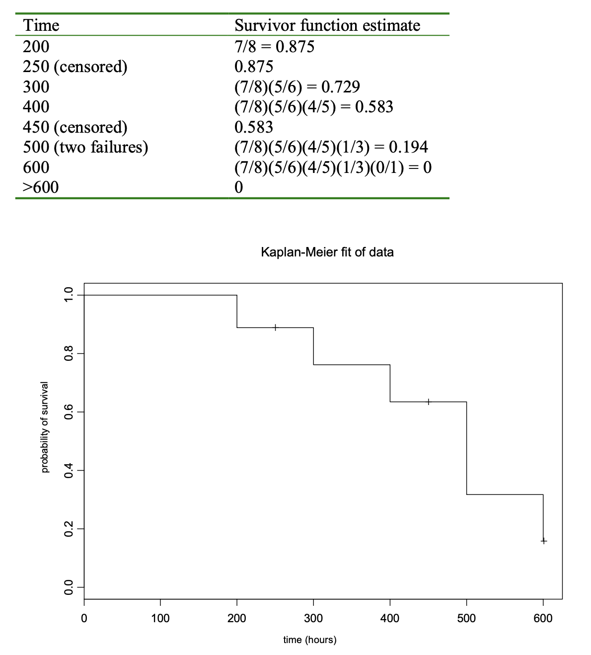
As an illustration, I will embellish on an example from a very good book, “Applied Reliability” by Tobias and Trindade. Suppose you have eight parts on test and the failure times are 200, 300, 400, 500 and 600 hours. Suppose due to a glitch, two parts are removed before failure at 250 and 450 hours. Also, let’s assume that two parts fail at 500 hours. The probability of survival past 200 hours would be approximately 7/8 = 0.875 since one part had failed right after that time out of eight total. At 250 hours, one part was removed although it hadn’t failed. It is a censored data point. So, just before 300 hours, there are six parts left. Then, the probability of lasting greater than 300 hours will be the probability of surviving past 200 hours and then surviving past 300 hours. This can be approximated by (7/8)(5/6) = 0.729.
You may see a pattern developing here. Each time you have a failure, you multiply by a fraction. The fraction is determined by the total at the start of the test, minus the number that are no longer on test after time t (failures and censored observations), divided by the number at risk of failure before t. A tie is taken into account in the fraction by the numerator. The following table should help show how the estimate is found. I should note that the estimates in the table are not truly the Kaplan- Meier estimates, since it uses a slightly different fraction. But the technique is similar. I have included a graph of the true Kaplan-Meier estimate for comparison. Luckily, most software packages dealing with reliability will calculate the Kaplan-Meier survivor curve for you.
Regression Techniques
Some of you may have heard the term “regression” before. If you haven’t, you can think of it as a method of fitting a line (or curve) to your data. We used regression in finding the estimate of the cdf to the Weibull distribution in E-Math News Vol.1 No. 5.
Suppose you run life tests under different conditions and want to predict the time to failure as a function of the experimental conditions. Is there any way of using regression to predict the time to failure? The short answer is yes. However, this is an advanced area of statistics. It requires a solid statistical background to understand and use in much depth. However, some understanding can be gained by treating the very simple case of one variable.
The usual equation for regression is
Y = b0 + b1x + s*eN
where Y is the response we are interested in, x is the variable we control in the experiment, b0 and b1 are the intercept and slope of the line, respectively, s is the standard deviation, and eN is the “error” or “noise” term. In the above equation, x, b0, b1 and s are considered fixed (not random) while Y and eN are random. So, you can use regression software to estimate the values of b0, b1 and s, thereby fitting a line to your data.
The s*eN term ends up “sprinkling” a little variation or noise on top of the line you fit, i.e. the line you fit does not go through each data point. You may have heard the term “constant variance assumption” in regards to regression. This comes from the above equation where the standard deviation (the square root of the variance) is considered constant.
When we get the estimates of b0 and b1 from software, we can predict Y for a given value of x. Of course, the s*eN term smears the prediction a little so we don’t get an exact value of Y. Instead, we estimate an average value of Y and put confidence limits on the predicted average. To see en example of how to do this, see E-Math News Vol. 1 No. 1.
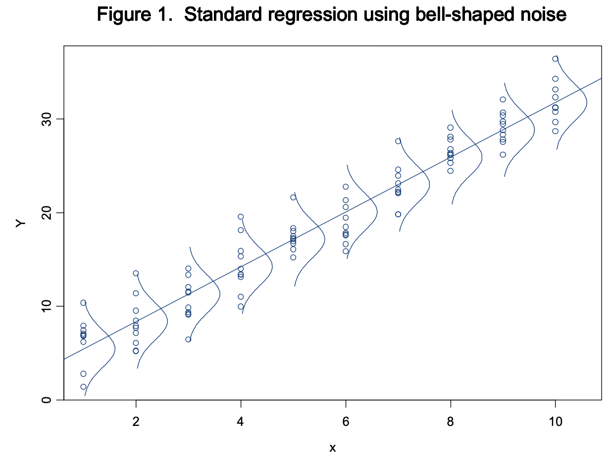
Before finding the confidence limits for Y, we need to know how s*eN is spread out (it’s distribution). Usually in regression, it is assumed that eN has a normal distribution (bell curve) with an average of 0 and a standard deviation of 1 (also called a standard normal distribution). It turns out that multiplying eN by the fixed value of s gives a normal distribution with an average of 0 and a standard deviation of s. Figure 1 shows a plot of hypothetical data using the standard regression technique. Note that the little bell curves demonstrate that the data are smeared out symmetrically about the line. So a change in x shifts the average value of Y, but doesn’t change the variation around that average.
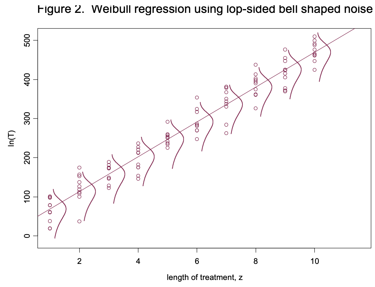
What do we do in the case of life data that follow the Weibull distribution? It turns out we can use a very similar technique, except that the noise is no longer bell shaped. Let’s say we are looking at the lifetimes of light bulb filaments, T, as a function of “length of treatment z”. The higher the value of z, the longer the life. Figure 2 is a plot similar to Figure 1. However, the noise term is different. It uses a lop-sided bell.
The equation we use is
ln(T) = a0 + a1z + v*eEV
where ln(T), a0, a1, z and v are analogous to Y, b0, b1, x and s respectively. Again, “ln” means natural log. So, if none of the data are censored, the log of the time to failure can be fitted to a straight line using standard regression software found in most statistics packages. If we want to put a confidence interval on the predicted value of ln(T), we can’t use the normal distribution. Instead, we use the distribution of eEV which has something called a “standard extreme value distribution.” In the standard regression case, the value of s is considered constant for all values of x. In the Weibull regression case, the value of v is fixed if the shape factor is constant for all values of z.
If any of the data are censored, then you can’t use the standard method to estimate a0 and a1. Instead, you have to solve a likelihood equation similar to the one discussed before. As I think you can see, using regression with the Weibull distribution is a little more involved than the standard regression case. Even so, I think this gives you a feel for how it is done. Luckily, many statistics packages do all the nasty calculations so you don’t have to.
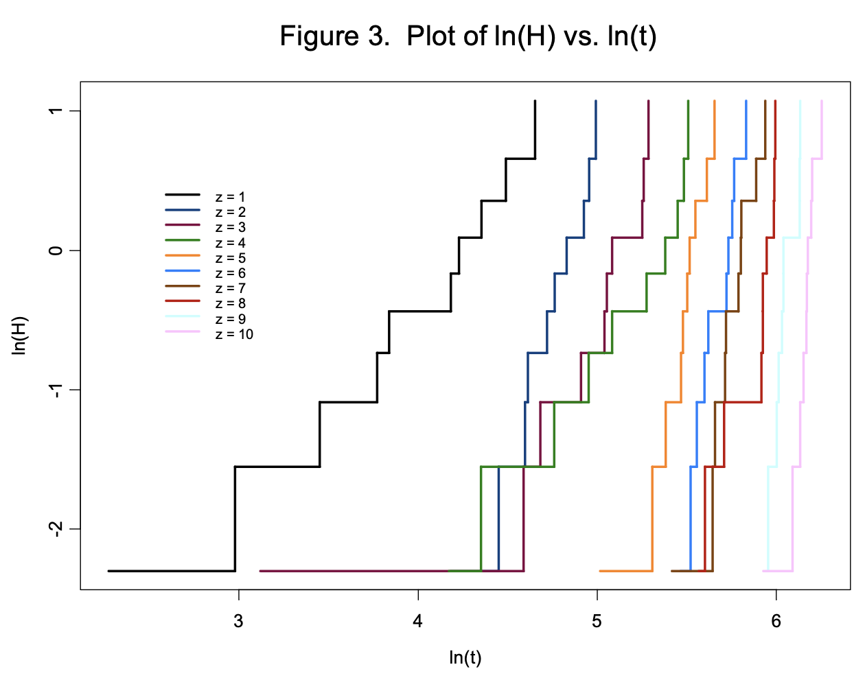
Lastly, there is a quick graphical check to make sure the Weibull model is appropriate. It turns out that a graph of ln(H) vs. ln(t) where H is the cumulative hazard (estimated using a non-parametric technique like the Kaplan-Meier) and t is the time to failure, should be roughly linear. Figure 3 shows a plot of ln(H) = ln{-ln[S(t)]} vs. ln(t) for each value of z in Figure 2, where S(t) is estimated using the Kaplan-Meier technique. Since the stair patterns for each group are fairly linear, the Weibull model appears justified. Note that the slopes of the lines are all about the same. This is because the shape factor in each group is the same. This is analogous to the standard regression case, where the treatment is considered to shift the mean, while the variance (or standard deviation) is constant. While the graph doesn’t “prove” that the Weibull model is correct, it appears at least that it “works”.
Summary
Many aspects of the Weibull distribution have been discussed. We have seen
- Several different functions that can be derived from the cdf,
- The importance of independent observations,
- The conditions under which the Weibull works best,
- The likelihood equation and how it handles ties and censoring,
- The distribution of the Weibull parameters a and b (which can be used to perform SPC),
- A way to estimate the survivor function without assuming any distribution at all (Kaplan-Meier estimate), and
- How to predict the time to failure using regression.
Whew! That’s a lot. While I have only touched on these subjects, I think I have provided you with at least a basic understanding. If you would like to know more, I encourage you to look into it in more depth and let me know if you have any more questions.