Using JMP to Create Experiment Designs with Non-Linear Constraints - Two Examples from the Pharmaceuticals Industry
Experiment Designs provide a powerful planning tool for effective experimentation. Some experimental situations have physical limitations, or constraints. JMP's Custom Designer provides for the inclusion of constraints in experiment designs. In this post you will learn two different ways to create Experiment Designs with non-linear constraints using JMP.
Introduction
People love to simplify. Nature is perfectly comfortable with complexity. In this paper you will see how to simplify Nature's complexity without losing your grasp on the real world.
Unconstrained Experiment Designs
Design of Experiments is a powerful Statistical technique for extracting the maximum amount of information from the minimum amount of experimental work. It is valuable in industry because it allows experimenters to balance frugality with thoroughness.
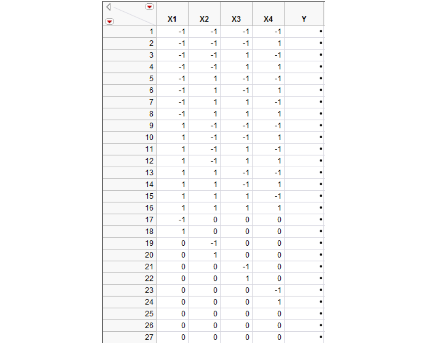
A typical designed experiment will vary a number of factors, each from a low to high level. If every combination of factor levels within these high and low limits is allowed, the design is “unconstrained.” The table below is an example of an unconstrained experiment design.
Linear Constraints
An experiment design is “constrained” when it has limitations on the combinations of the factor levels. These limitations come from aspects of the real world.
If these limitations can be expressed mathematically as the sum of scaled factor levels, the constraint is called “linear.”
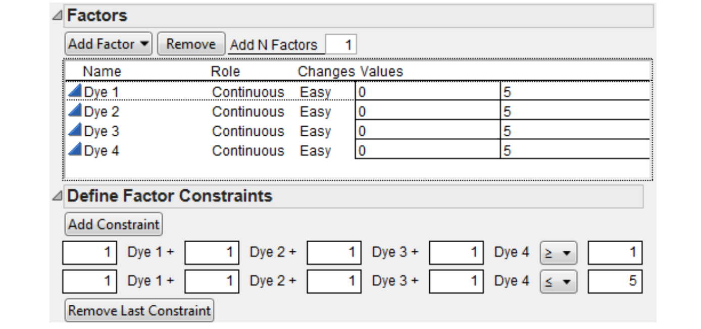
For example, suppose you want to study combinations of dyes in an ink-jet ink. Each dye can range from 0 to 5% in the ink, however the total amount of dye must be at least 1% in order to be seen and no more than 5% to prevent nozzle clogging.
Mathematically the constraints look like this:
%Dye1 + %Dye2 + %Dye3 +%Dye4 > 1%
*%Dye1 + %Dye2 + %Dye3 +%Dye4 < 5%
Clearly an unconstrained experiment design will not work for us here. For instance, it will ask for a combination of dyes that is 5% of each, or 20% total dye. Similarly it will ask for an ink that has no dye at all.
JMP's Custom Designer let's us specify these linear constraints as shown below.
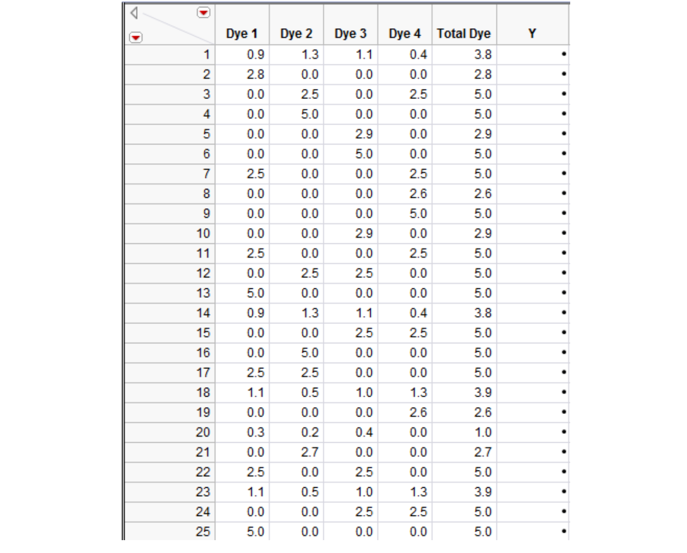
The table below shows a design created for these constraints. The "Total Dye" column has been added to check that the constraints are satisfied, i.e., the total concentration of dye is between 1% and 5%.
Non-Linear Constraints
Human beings prefer linear constraints because they are easier to deal with. Nature does not share this preference. The real world has many nonlinear constraints.
An example of a nonlinear constraint would be when factor levels are multiplied. For example, suppose you were studying current and resistance, among other factors, and you had a requirement to keep the voltage between two levels, Elow and Ehigh. The constraints would look like this:
I X R > E_low
I X R < H_high
The remainder of this paper will examine three examples of nonlinear constraints and how JMP's Custom Designer can be used to create experiment designs to obey them.
A Simple example: Laser Drilling
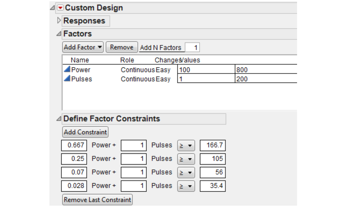
A medical equipment manufacturer needs to drill holes in polymer parts with a pulsed laser. They want to use a designed experiment to study the Number of Pulses and the Laser Power to optimize the quality of the holes drilled. They are interested in 13 to 200 pulses and power from 100 to 800 mW.
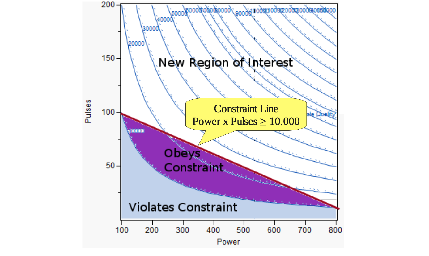
Holes cannot be drilled if the product of pulses and power is less than 10,000–the material is not penetrated. Thus, this experiment has a nonlinear constraint:
Power X Pulses > 10,000
One way to create the necessary design would be to generate the unconstrained design and adjust it to obey the constraint. With this simple situation that would be easy–you would only need to adjust the low, low trial (100, 13), possibly to (100, 100) as shown below. The red line shows the new region of interest created by adjusting the low,low corner to obey the constraint. Notice that many combinations of Power and Pulses that obey the constraint are outside the new region of interest.
In order to include more legitimate combinations in the region of interest, we can approximate the nonlinear constraint with several linear constraints, as shown below.
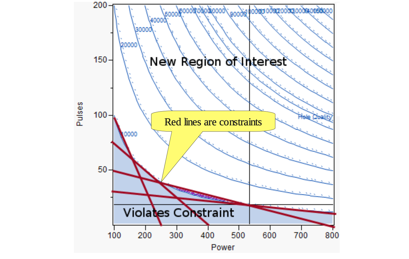
Notice that with four linear constraints, we include nearly all of the legitimate Power-Pulse combinations. Specifically, the constraints are:
Constraint 1: (0.667 X Power) + Pulses ≥ 166.7
Constraint 2: (0.25 X Power) + Pulses ≥ 105
Constraint 3: (0.07 X Power) + Pulses ≥ 56
Constraint 4: (0.028 X Power) + Pulses ≥ 35.4
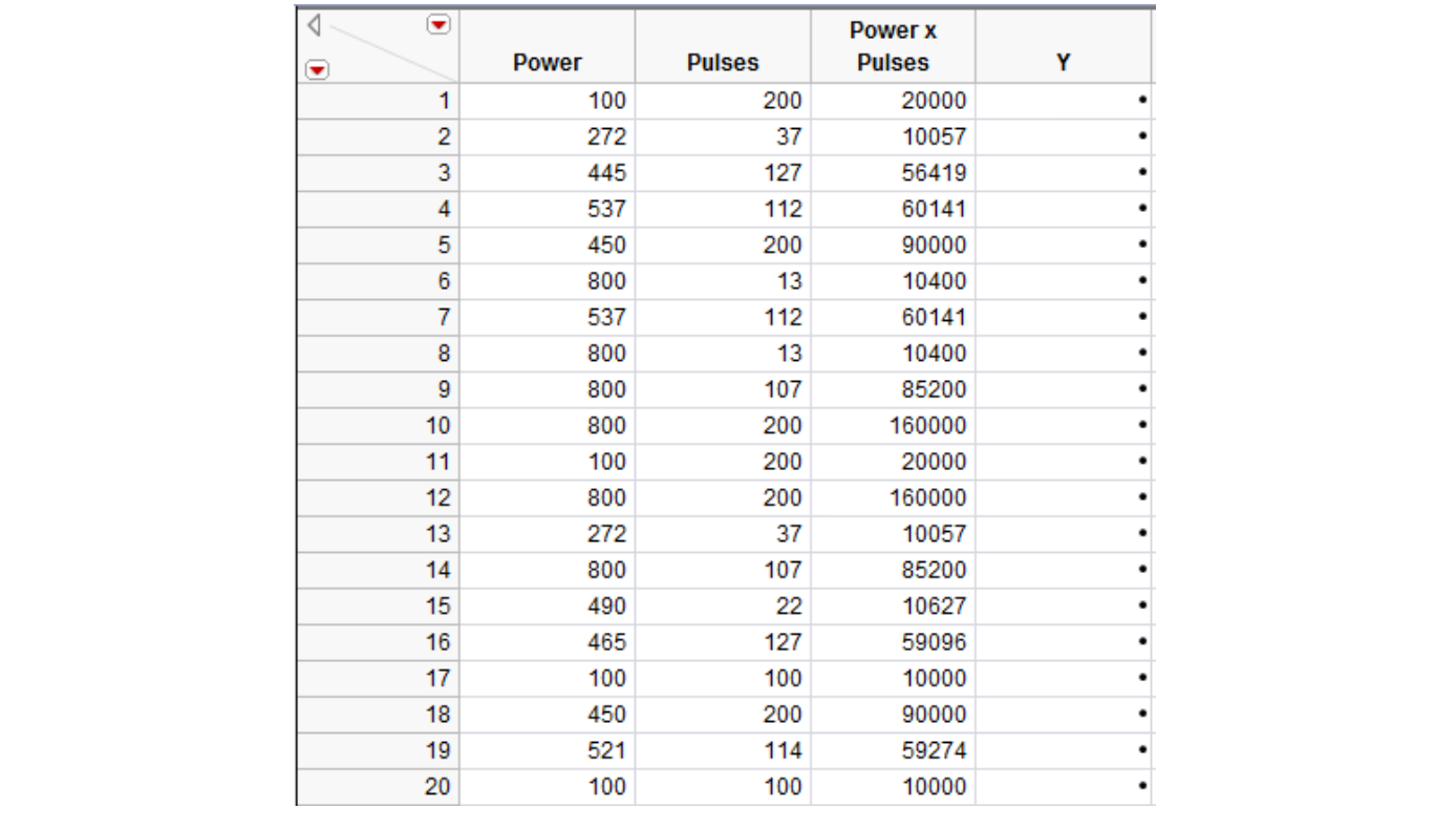
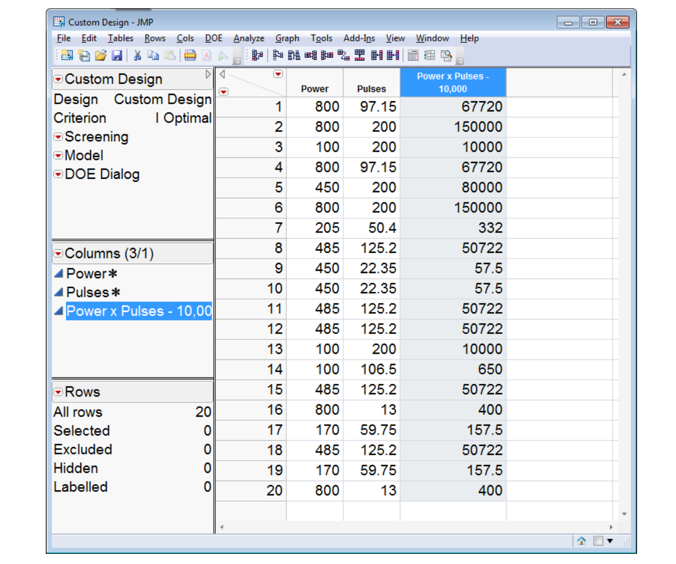
These are specified in JMP as shown below along with the experiment desing created with these constraints.
JMP can handle non-linear constraints directly. My friend Brad Jones showed me how. First, select “Disallowed Combinations” from the red triangle drop down menu in the Custom Design module.

Enter the non-linear constraint in the “Enter Expression” window. Please notice that this must be entered differently from a linear constraint. Linear constraints are allowed – these are “Disallowed Combinations.”
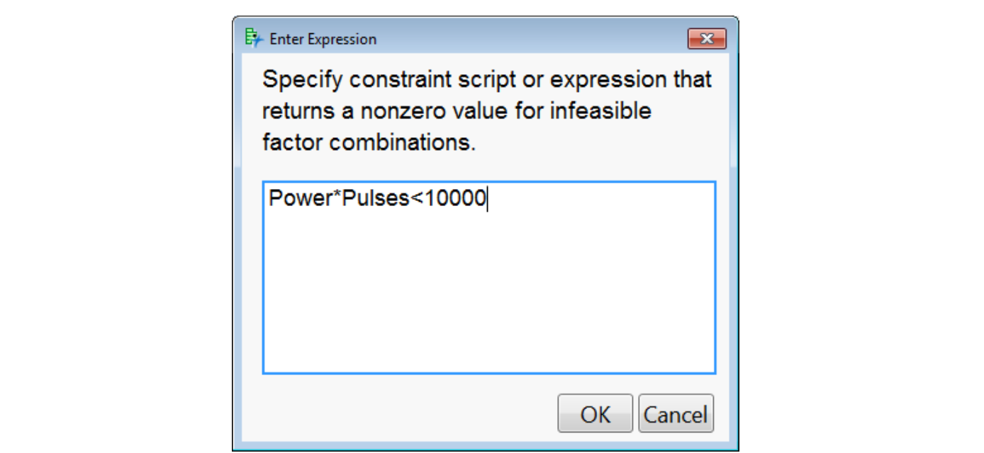
Click "OK," and then JMP will build the experimental design with the specified constraint.
A More Complex Example: A Known Constraint – Osmolality
Igenica needs to to optimize an injectable formulation for shelf-life. The factors are:
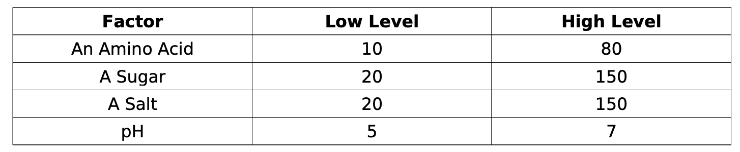
The optimal formulation must have an osmolality between 270 and 330 mOsmo (osmolality measures the body's electrolyte-water balance). A formulation outside this range will cause pain when injected. Ideally our formulation will be as close to 300 mOsmo as possible, so the goal will be to stay between 295 and 305 mOsmo.
Here is the mathematical expression of this constraint:
Osmolality = A.A.Multiplier X [Amino Acid] + [Sugar] + 1.86 X [Salt]
A.A.Multiplier X [Amino Acid] + [Sugar] + 1.86 X [Salt] > 295
A.A.Multiplier X [Amino Acid] + [Sugar] + 1.86 X [Salt] < 305
Now for the complication: the value of the A.A.Multiplier changes with pH. Paul had his team study this phenomenon. The results in the table below show experimentally determined values of A.A.Multiplier for different pH values.

A Least Squares fit to these data yields,
A.A.Multiplier = 3.808 - 0.396 X pH
Substituting this in our constraints gives,
3.808 X [Amino Acid] - 0.396 X pH X [Amino Aicd] + [Sugar] + 1.86 X [Salt] > 295
3.808 X [Amino Acid] - 0.396 X pH X [Amino Aicd] + [Sugar] + 1.86 X [Salt] < 305
The term for pH x [Amino Acid] makes these nonlinear constraints since pH x [Amino Acid] is the product of two factors. Bill had to simplify these in order to create an experiment design with JMP.
The first thing to try might be creating an unconstrained experiment design and adjusting the levels that violate the constraints. Unfortunately, this only results in tremendous tedium and frustration!
Maybe approximating the constraint with several linear constraints would work, as it did for the Laser Drilling example. Of course this problem has more factors, so constraint planes (or more accurately, constraint hyperplanes) would be needed instead of lines. Isaac Newton may have found this relaxing, but it is completely impractical for most of us.
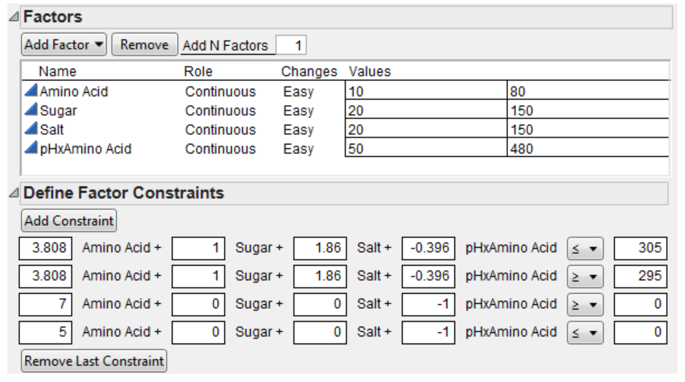
Fortunately there is a trick that simplifies this constraint without pain. Instead of using pH as a factor, use pH x [Amino Acid] as the factor. This instantly converts our constraints into linear constraints! This new factor will now require two linear constraints of its own to keep the pH in range, namely,
7 X [Amino Acid] - pH X [Amino Acid] ≥ 0
5 X [Amino Acid] - pH X [Amino Acid] ≤ 0
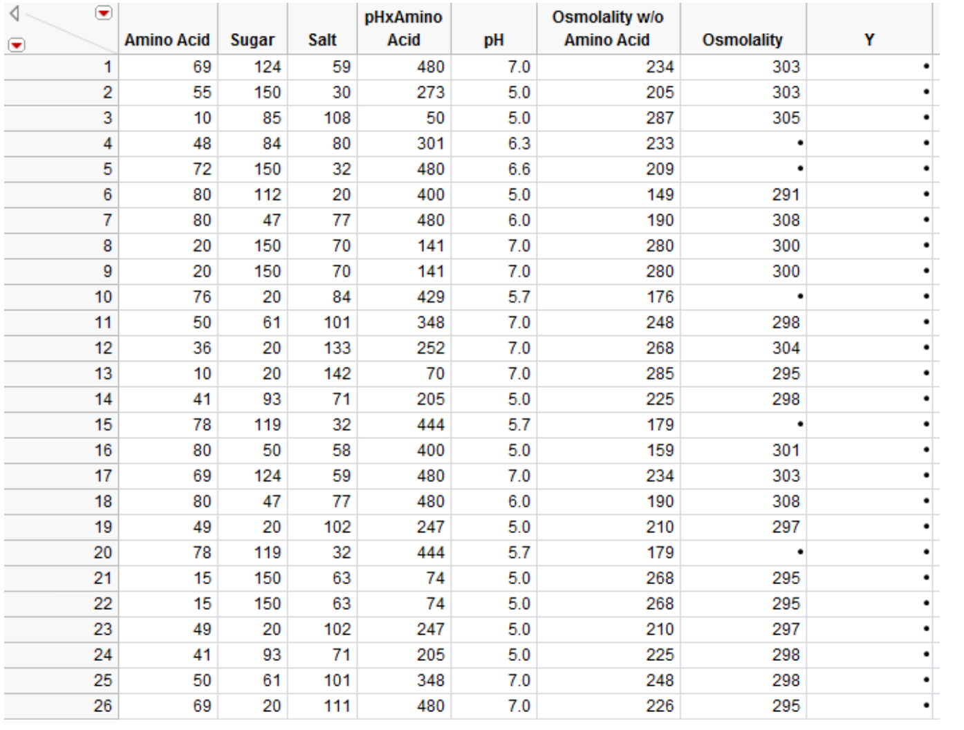
These constraints specified in JMP and the resultant experimental design are shown below. A column for pH has been added to make this easier to run in a lab. Some osmolality values are missing because no experimental value for A.A.Multiplier was available at these pH values. Notice that the calculated osmolality deviates slightly from the constraint, but is well within an acceptable range with no adjustment.
An Even More Complex Example: An Unknown Constraint – Solubility
Alder Biopharmaceuticals produces antibodies for pharmaceutical use. Antibodies can target a variety of maladies from arthritis to cancer. These antibodies are produced by yeast cells that live and grow in a fermentation medium.
Patti needed to optimize this fermentation medium. The formulation had 5 salts (factors) that needed to be optimized, namely A, B, C, D, and E. It was important that every formulation in the experiment be soluble, i.e. form no precipitate.
In the last example, Paul had a table expressing the osmolality constraint. In this example, no such table existed for the solubility constraint. Even worse, there was no theory strong enough to formulate a mathematical constraint.
What to do?
Patti came up with a great idea – develop an empirical model of the solubility to define the constraint. This approach required two experiment designs. The first experiment design was needed to build a solubility model which could be used to define the constraint needed for the fermentation medium formulation design. A second design was needed, incorporating the constraint defined with the first design, to optimize the fermentation medium formulation.
Defining the Constraint: The Empirical Model for Solubility
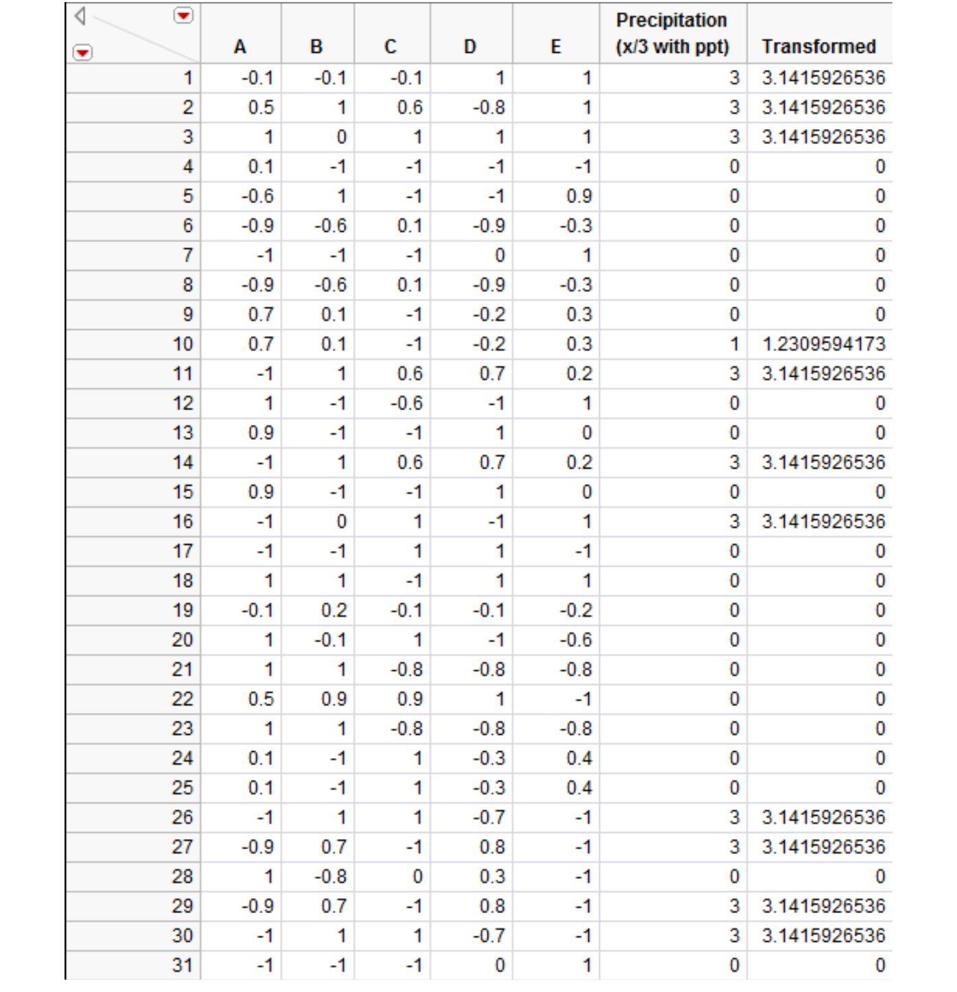
The first design was very straightforward. All of the ingredients were relatively small additions to a bulk medium, so an unconstrained I-Optimal design was used. Three samples were prepared for each run in the design. The response was the number of samples forming a precipitate (ppt). The standard transformation for proportions was used to meet the assumption of constant Standard Deviation:
2 X arcsin(sqrt(Y/3))
The empirical solubility model is,
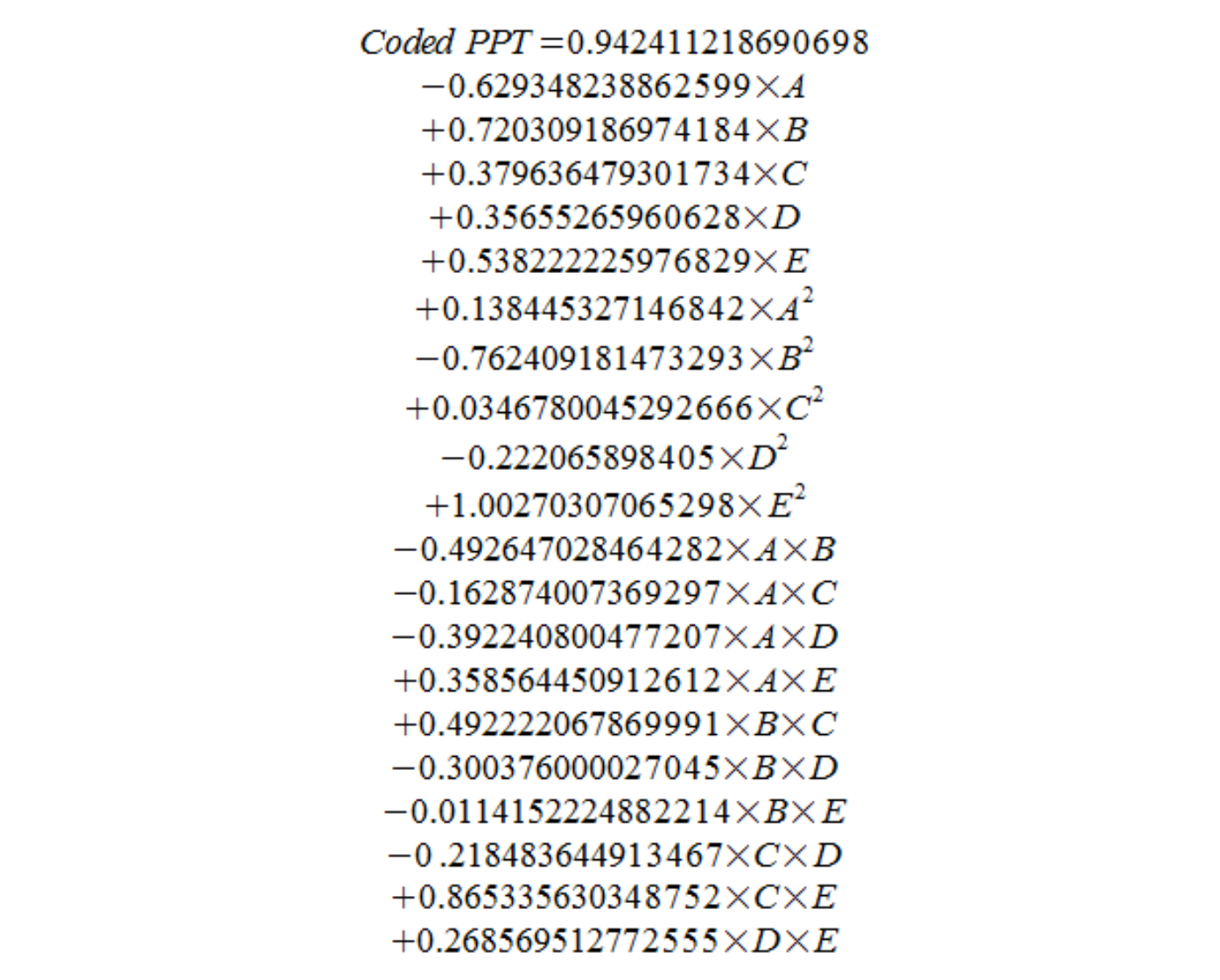
This is very helpful, but extremely cumbersome to work with directly! Where would we be without JMP? Fortunately JMP makes it easy to plot a variety of different views of the data, simplifying the job of working with this highly nonlinear constraint.
Optimizing the Fermentation Medium: The Second Design
The second design needed to optimize the salt concentration to make the best yeast fermentation medium. The first requirement is that the design ask for no salt combination that would form a precipitate, so Predicted PPT must be 0.
Patti decided to hold E constant at -1 for the second experiment. Her reasons had nothing to do with the results seen so far. To keep things manageable, a new design with just the 4 salts of interest (A–D) was created. A column was added for E with -1 for every run because it is needed in the formula. A column was created for the response “Coded PPT” by pasting the column properties from the original experiment (nicely bringing the formula along for the ride!). Finally, a column for the uncoded prediction of PPT was created by using a formula to reverse the transformation.
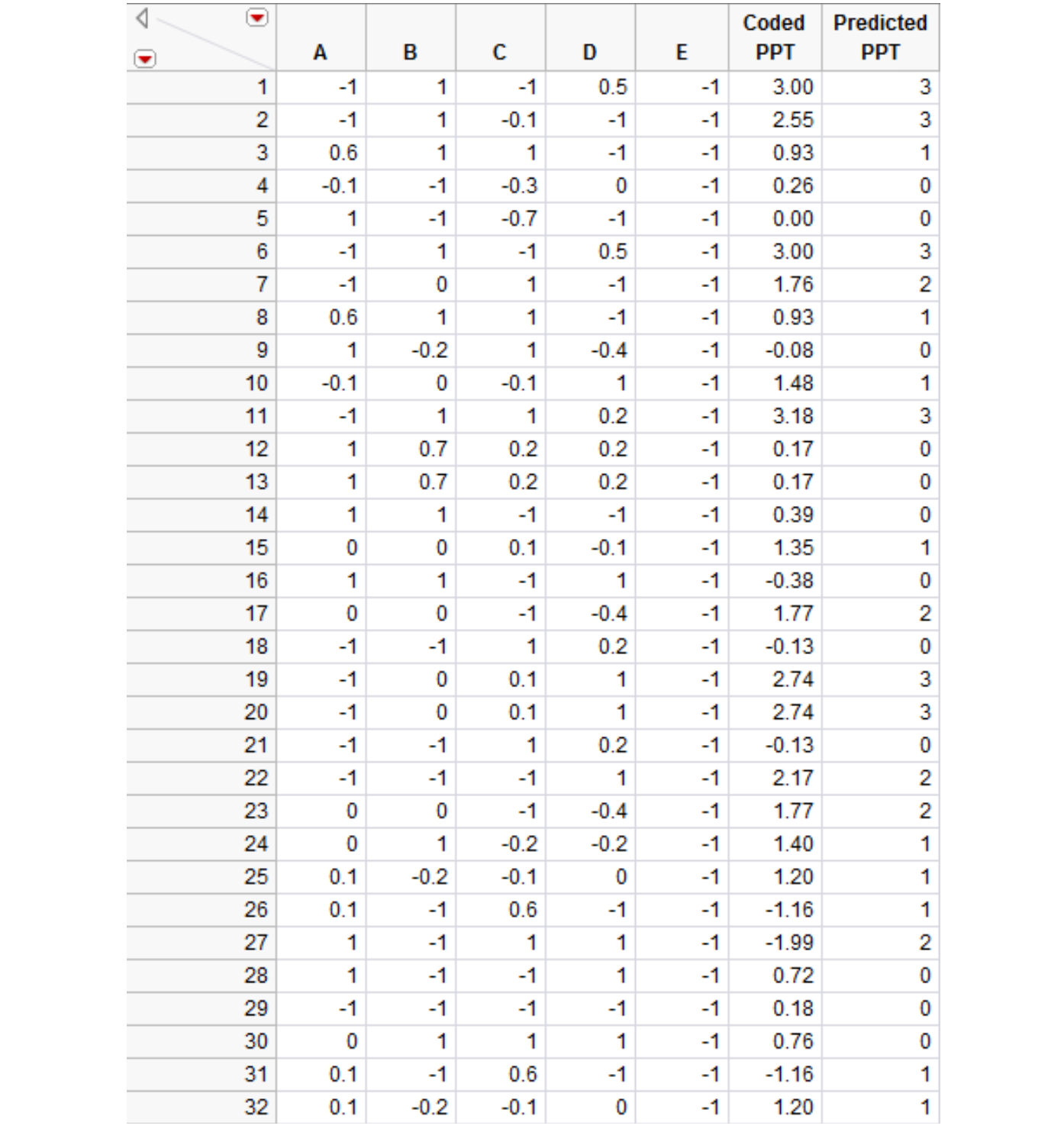
We are seeking zero Predicted PPT so, as you can see in the table above, an unconstrained design is impossible – too many runs show predicted precipitation of 1, 2, or 3 and we must have 0.
Bill needed to find linear constraints to approximate the model for Coded PPT. To simplify this procedure he decided to look for linear constraints on two factors at a time. This made it possible to use lines for the approximation, just as was done in the Laser Drilling example.
Initially, JMP's Graph Builder was used to decide which two-factor pairs might make sense to work with. Many graphs suggested interactions. B and D were chosen for the initial factor pair. The graph below shows that the right combination of B and D is critical for success. Only this combination produces Low Predicted PPT

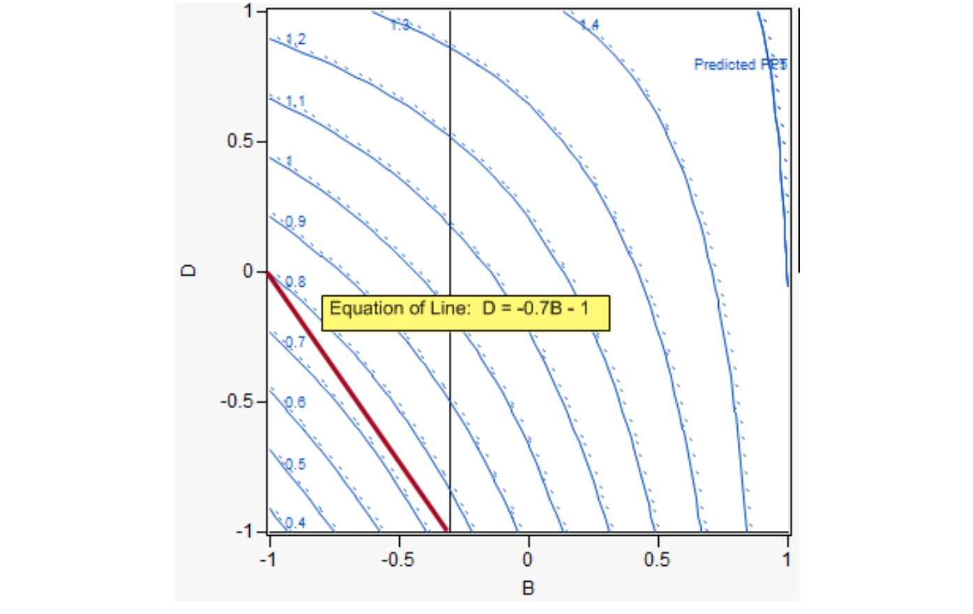
Next, this model was fitted:
Y = B0 + (B1 X B) + (B2 X D) + (B12 X B X D)
A contour plot of B vs D is shown below. The red line is a linear constraint to keep the Coded PPT less than 0.8 (equivalent to 0.5 ppt out of 3 ). A design created with only this constraint was still unacceptable because it had many trials with Predicted PPT of 1 or greater.
Next Bill used JMP's Stepwise Regression to give further clues as to the appropriate factor pairs to consider for the next constraint line.
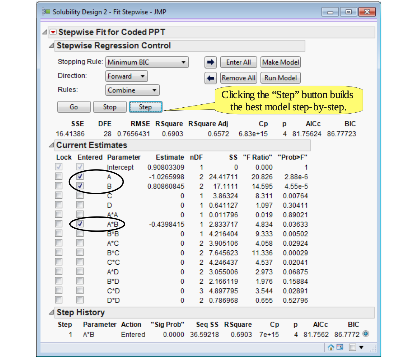
This regression indicated the model:
Y = B0 + (B1 X A) + (B2 X B) + (B12 X A X B)
A contour plot of A vs B is shown below. The red line is a linear constraint as before.
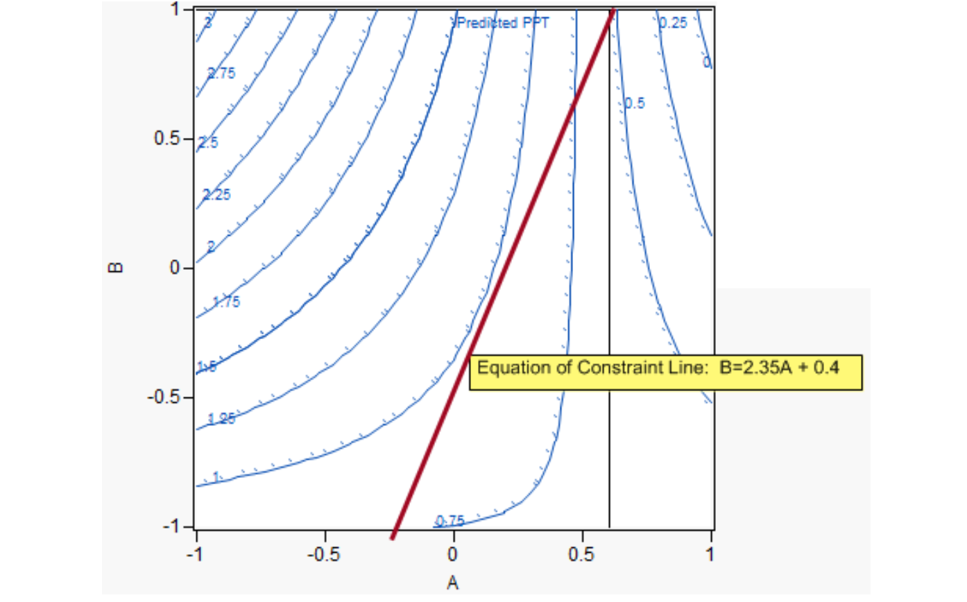
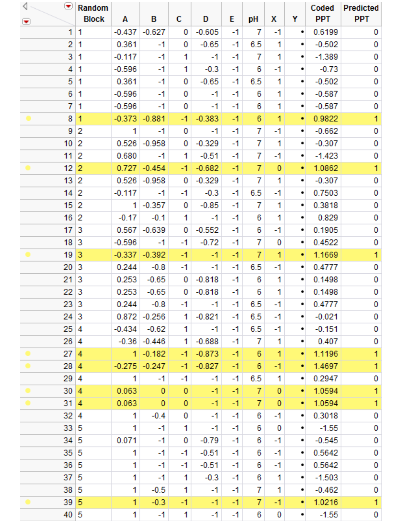
An acceptable design was created using these constraints:
(-2.35 X A) + B ≤ 0.4*
(0.7 X B) + D ≤ -1*
This design is shown in the table below. The rows highlighted in yellow still showed precipitate and needed to be adjusted. additional hand adjustment was required. The
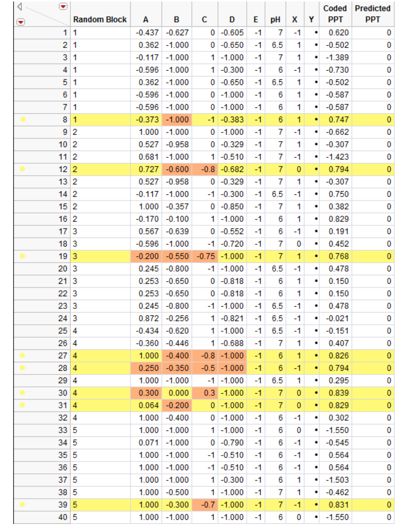
The final Fermentation Medium Optimization design after adjustment is shown below. Adjusted levels are highlighted in orange.
Conclusion
Nature is complex. Some experimental situations have physical limitations, or constraints. Some experiments have non-linear constraints, and these are more difficult to work with. JMP's Custom Designer provides for the inclusion of both linear and non-linear constraints in experiment designs. In this post you have seen how to use JMP's "Disallowed Combinations" feature to add non-linear constraints. You have also learned how to simplify complicated non-linear constraints that were too extreme to work with the "Disallowed Combinations" feature directly.
About the Authors
Paul Sauer is Vice President of Process Sciences & Manufacturing at Igenica. He is responsible for the development and manufacture of monoclonal antibodies for use in pre-clinical and clinical oncology studies.
Patricia McNeill is Head of Research Fermentation at Alder Biopharmaceuticals and is responsible for helping to advance Alder's Mab Xpress technology for producing therapeutic antibodies in yeast.
Bill Kappele is President of ObDOE. He is responsible for course delivery and development. Paul and Patti both learned Design of Experiments from Bill.